📖 Day 5 – Financial Statistics
Rolling Statistics: Moving Average
This day I explored rolling statistics in Pandas, applied to financial time series; this lets me smooth data and analyzing volatility trends.
Main Goals:
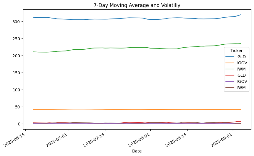
- Calculate moving averages (in this work 7 days) of closing prices.
- Calculate standard deviation (volatility), so the risk of each asset.
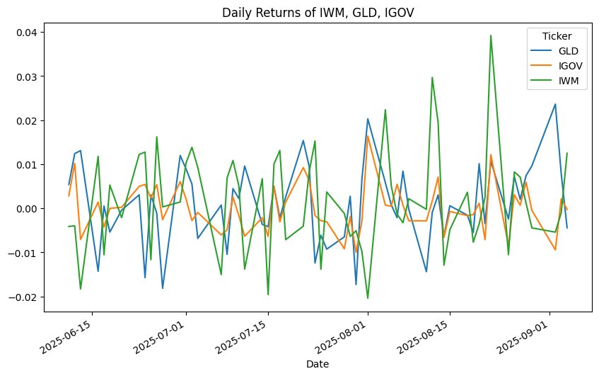
- Plot: first plots of daily returns and rolling metrics
Step by Step
📍 Step 1: Download of data Matrix with assets and volumes as per previous works (closing prices and volumes of IWM, GLD, IGOV).
📍 Step 2: Calculated .pct_change(), 7-day moving average, and rolling std.
📍 Step 3: Plotted returns, moving averages, and volatility together, comparing the performances of each asset.
Challenges / Insights
- Learned how .rolling(window) works.
- Discovered how to layer multiple plots on the same figure (ax=plt.gca()).
- Saw how volatility clusters can appear visually.
Code Snippet
```python
returns = close.pct_change().dropna()
mov_avg = close.rolling(window=7).mean()
std = close.rolling(window=7).std()

returns.plot(figsize=(10,6), title="Daily Returns")
mov_avg.plot(figsize=(10,6), title="7-Day Moving Average")
std.plot(ax=plt.gca())
plt.show()

```
Plots
Next Step
👉 Correlation analysis between assets.