📖 Day 6 – Data Cleaning
Handling values in a Dataset
Today I focused on cleaning financial time series data and exploring basic descriptive statistics with pandas. Handling missing values and computing summary stats are essential skills before moving to more advanced financial models, and to make the basic statistics working.
Main Goals:
- Handle missing values (NaN) in time series data, removing or replacing them
- Compute descriptive statistics (mean, std, min, max, etc.)
- Price normalisation for easier comparison
- Calculation of rolling mean and standard deviation
Step by Step
📍 Step 1: Sample DataFrame creation with fill() or drop functions to handle missing values (NaN);
📍 Step 2: Download 90 days of a ticker group of 3 assets (IWM, GLD, IGOV), using functions to fill or eliminate the missing values (.ffill() or dropna())
📍 Step 3: Descriptive statistics calculation through the .describe() function, and rolling mean and std calculation
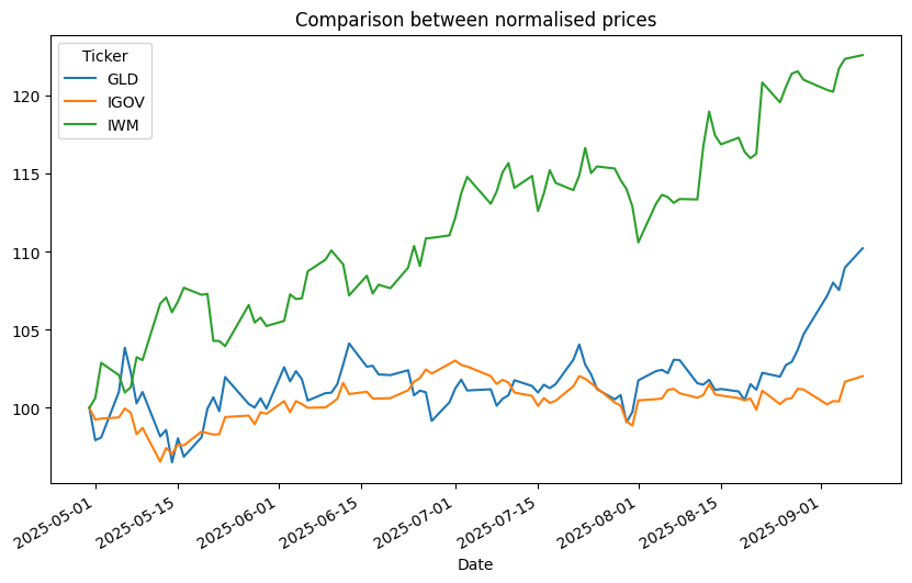
📍 Step 4: Normalisation of time series (all assets start at 100), and plotting for data visualisation.
Challenges / Insights
- Learned that pandas fillna(method=”ffill”) now raises a deprecation warning → better to use .ffill().
- Realized normalization is useful, especially in the comparison between assets with consistently different price scales.
- Rolling standard deviation gave an immediate sense of volatility dynamics across tickers.
Code Snippet
```python

# Step 2: Check and fill missing values
print("Missing values per asset:\n", close_prices.isna().sum())
close_cleaned = close_prices.fillna(method = "ffill")

# Step 3: First Descriptive stats
print("\nDescriptive Statistics:\n", close_cleaned.describe())

# Step 4: Normalise values (starting from first Value = 100)
normalized = close_cleaned / close_cleaned.iloc[0] * 100
print("\nNormalized Prices:\n", normalized.head())


```
Plots
Next Step
👉 Data Visualization with matplotlib & seaborn: comparing returns, correlations, and building clearer insights through plots.